SYS-0006 — Virtual sensor drift detection
| Status | verified — engine e2ff2f8, cxf:fnv1a128:7b8d5126bff08106d7dae20ea85ecc3c, 2026-08-17 |
| Severity | 3 |
| Method | statistical |
| Phase | 2 |
| Category | COMFORT_ENERGY |
| Confidence | LOW |
| Estimation | QUALITATIVE_ONLY |
| G36 | — |
| Clusters | CLU-09 |
| Suppresses | — |
| Suppressed by | — |
| Related | SYS-0005, SYS-0009, SYS-0010, AHU-0028, RTU-0003 |
| Playbooks | sensor-drift |
| Source | HVAC FDD Reference v1.0 §16, SYS-0006 (pdf pp. 144-145) — the residual equation, both published thresholds, the four diagnoses, the whole impact profile, and the Koo & Yoon note; The reference’s own provenance line for that card: Koo & Yoon 2022; Sun et al. 2024 (virtual sensor RMSE 0.30 °C, bias > 1 °C detected reliably); Accepted design: internal sensor-health design note (local-only, not distributed) (§2 stance, §2.3 the adjudicates contract, §4.3 the MovingAverage ring floor, §4.4 vector strategy); Library precedent: SYS-0005 (the pair form of the same question), SYS-0009/SYS-0010 (the role-point sensor family), AHU-0022 (Reals.MovingAverage at a 64-checkpoint ring), HP-0001 and VAV-0001 (host-fitted baselines consumed as ordinary points) |
| Operating states | all, within the operating envelope the virtual sensor was trained on. The graph has no gate and evaluates whenever the host publishes a prediction, so the envelope is the host’s to enforce: a Ridge model fitted over a summer learning period is extrapolating in January, and its extrapolation error arrives here as a residual indistinguishable from sensor drift. Where the host cannot vouch for the prediction it should stop publishing virtual_value rather than publish a guess. |
Preconditions (host-enforced): physical_sensor and virtual_value are a ROLE PAIR, not canonical names: the host’s instance configuration records which real point physical_sensor is bound to, and that record is what resolves this card’s adjudicates target. Both thresholds are in the BOUND point’s units — the reference’s 1.5 and 3.0 are its temperature defaults and MUST be retuned for any other quantity kind. Four host obligations decide whether this rule means anything. (1) The model must never take the accused sensor as one of its own features: a regression that can see physical_sensor predicts it perfectly, the residual collapses to zero, and the rule goes permanently silent while reporting health. (2) The learning period must be known-good. A model trained while the sensor was already 2 K high learns the bias as truth, and the drift becomes invisible from the moment it is fitted — this rule cannot detect a fault that predates its own baseline. (3) Model health is a separate question with a separate rule: the reference’s META-FC-050 (statistical model confidence degradation) is what says the Ridge fit has stopped tracking, and a host running it should read a degraded model as NO_EVAL here rather than as sensor drift. (4) Delivery quality is resolved before this rule runs, not by it — a value held over from a dead subscription reads as a residual, and the rule is right about the number it was given and wrong about the sensor (design doc §2.2). Recommended: report NO_EVAL for the first
windowafter load, where both statistics are computed over a partial window; the graph will still produce a verdict there, andbias_present_at_loadpins what that verdict looks like.
Points: physical_sensor, virtual_value
Outputs:
yFault— True once the residual has broken either the bias band or the noise band continuously for alarm_delay. While true, the host treats physical_sensor as invalid for every rule bound to this equipment instance that consumes it (see adjudicates), weighed against diagnosis 4yBias— Sub-condition flag, undelayed — the window mean of the residual is outside bias_threshold. True with yFault means diagnosis 1 (calibration drift). Not an evaluability output: a false yBias never means NO_EVALyNoise— Sub-condition flag, undelayed — the window variance of the residual is above noise_threshold squared. True with yFault means diagnosis 2 (intermittent failure). Not an evaluability output
Parameters:
| Name | Default | Unit | CXF path | Description |
|---|---|---|---|---|
bias_threshold | 1.5 | varies (the bound point’s own units) | biasHigh.t | How far the window-mean residual may sit from zero before the sensor is accused of a calibration bias. The reference’s 1.5 °C, which sits above the ~1 °C floor Koo & Yoon report this method detects reliably and above the 0.30 °C RMSE of their model. PER-BINDING: it is a temperature number, and a pressure or humidity binding needs its own. |
noise_threshold | 3.0 | varies (the bound point’s own units) | noiseThr.k | Residual standard deviation above which the sensor is accused of intermittent failure rather than bias. The reference’s 3.0 °C, published in natural units and kept that way — the graph squares it internally (see Deviations), so a host retunes noiseThr.k in degrees and never in degrees squared. PER-BINDING, same caveat as bias_threshold. |
window | 3600.0 | s | muResid.delta, muSq.delta | Rolling window both statistics are computed over (60 min). LIBRARY-CHOSEN — the reference’s tunables line is truncated in the source pdf and publishes no window. One card parameter binds both MovingAverage instances and hosts must set them together; a host ticking faster than window/63 (57.1 s at the default) silently shortens the window through the block’s 64-checkpoint ring. |
alarm_delay | 1800.0 | s | persist.delayTime | Continuous persistence required after either branch trips before the alarm asserts (30 min). LIBRARY-CHOSEN for the same reason as window; 30 min is the AlarmDelay the reference publishes for its sibling sensor rule SYS-0005. |
Description
Give a sensor a second opinion built from every other point that correlates with it, and the difference between the two is evidence the sensor cannot supply about itself. That second opinion is the virtual sensor: a Ridge regression the host fits over a learning period on three or more correlated features, publishing a prediction of the accused point every tick. Koo & Yoon (2022) report an RMSE of 0.30 °C for that kind of model and reliable detection of biases above about 1 °C, which is the basis for putting a 1.5 °C band around the residual and believing what crosses it. The graph does two statistics on that one signal: the window mean, which catches the slow monotone bias, and the window variance, which catches the transmitter that has started jumping — the reference’s diagnoses 1 and 2, kept separable in the output rather than merged.
The adjudicates contract. While yFault is active, physical_sensor is
invalid: the host must return NO_EVAL for every rule on this equipment instance
that consumes it, deriving that set by intersecting each card’s points with
adjudicates.points. The verdict is invalid_while_active rather than
SYS-0005’s ambiguous because the rule names one sensor — its two inputs are
not interchangeable, one being a measurement and the other a computation — and
it is weighed against diagnosis 4 before acting.
Detection Logic
residual = physical_sensor − virtual_value

yBias  = |MovingAverage(residual, window)| > bias_threshold
yNoise = MovingAverage(residual², window) − MovingAverage(residual, window)²
                                          > noise_threshold²
yFault = (yBias OR yNoise) held continuously for alarm_delay
Block graph (rule.cxf.jsonld):
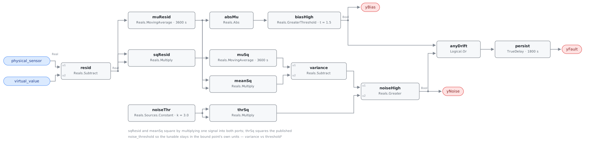
Thirteen blocks, one subtraction and two branches off it. The noise branch is
the identity Var(r) = E[r²] − (E[r])² built from blocks that exist: sqResid
squares the residual by feeding it into both ports of a Reals.Multiply, muSq
averages that, meanSq squares the mean the bias branch already computed, and
variance subtracts. noiseThr/thrSq do the same to the threshold, which is
why the published tunable stays in the bound point’s units — retune noiseThr.k
to 2.0 °C and the graph compares against 4.0.
Both comparisons are strict, as the reference writes them: a steady residual of exactly 1.5 reads healthy forever, and so does a square wave of amplitude exactly 3.0, whose variance is exactly 9.0.
The window is memory, and it cuts both ways. Reals.MovingAverage is a
continuous-time integral mean, so the statistics migrate rather than jump: a 2.5
bias appearing after a clean hour takes 0.6 of a window (1.5/2.5) to drag the
mean across the band, and the same arithmetic runs backwards after a repair. A
host expecting the finding to disappear the moment the technician closes the
ticket will conclude the repair failed.
The warmup convention is the exception to that patience: until the window fills,
MovingAverage divides by elapsed time rather than by the window, so a bias
already present when the controller starts is in the mean within one tick and
the alarm lands one alarm_delay later. persist asserts at exactly
T + delayTime and the disjunction must be held continuously — a branch that
trips and drops resets the timer. delayOnInit = true (CDL default false) on
persist.
Possible Diagnoses
The reference’s four, in its order:
- Target sensor calibration drift (bias error) — what
yBiasnames: a transmitter reading a fixed amount high or low, with nothing about it that looks broken - Target sensor intermittent failure (noise increase) — what
yNoisenames: the reading still averages correctly and has stopped being steady (a failing A/D channel, a loose terminal, an element on its way out) - Target sensor wiring degradation — presents either way: a corroded splice adds a bias, a marginal connection adds noise, and one cable can do both
- Correlated sensors have drifted (cross-check) — the residual is a difference and this rule attributes all of it to the accused sensor, because that is the only point it was pointed at; a drifted model input produces an identical output with the accused transmitter in perfect health
Diagnosis 4 is the residual ambiguity to weigh against invalid_while_active.
The cheap discriminator is the family: run SYS-0005, SYS-0009 and SYS-0010
on the model’s input sensors, and a clean bill on the features turns this
rule’s finding from a suspicion into an accusation. The expensive one is a
reference instrument, which is where the playbook ends up anyway.
Energy Impact
COMFORT_ENERGY, LOW confidence, QUALITATIVE_ONLY — the reference’s profile. There is no runtime waste term and this card does not invent one: a drifted sensor spends nothing by drifting. The cost is entirely cascade, through EEM-01 (sensor recalibration) and the downstream faults a believed-but-wrong reading causes or hides, and it is accounted for by the rules this one adjudicates. Confidence is LOW for a structural reason: the statistic is sound and its detection floor is published (near 1 °C of bias against a 0.30 °C model RMSE), but the verdict rests on a model that rests on other sensors and on a learning period nobody in the graph can audit. Diagnosis 4 is a standing false positive with no in-rule remedy; a model fitted on an already-drifted sensor is a standing false negative.
Emissions Impact
Scope 1 or 2 depending on what the mis-measurement drives, QUALITATIVE_EMISSIONS,
LOW confidence, avoided-emissions basis N/A — the reference’s assignment. The
ambiguity in scope is real: a drifted sensor biasing a boiler is Scope 1, the
same sensor biasing a chiller or economizer is Scope 2, and the sensor itself
emits nothing. The quantity is entirely cascade, which is why
runtime_estimation is empty.
Deviations
- The Ridge regression is host-side and never enters the graph. The
reference’s equation begins
virtual_value = regression_model.predict(correlated_features), none of which is expressible in CDL elementary blocks; the prediction arrives as the derived role pointvirtual_value, the same way HP-0001 and VAV-0001 consume host-fitted baselines. The consequence is that the correlated features are invisible here — the rule binds two points where the reference names four or more, which is exactly why diagnosis 4 is invisible to it. rolling_stdbecomes variance against the squared threshold. The engine has no standard-deviation block, butVar(r) = E[r²] − (E[r])²is buildable andvariance > threshold²is equivalent tostd > thresholdfor non-negative quantities. Publishingnoise_threshold_sq = 9.0and skipping two blocks was rejected: the reference publishes 3.0 °C, and a tunable in degrees-squared is hostile to whoever retunes it on site.- Sibling note, not an edit: AHU-0022 states that squaring inside a moving average is not expressible in this block set and substitutes mean absolute deviation. This card shows the variance form is expressible; whoever owns AHU-0022 should reconcile the two, though the MAD substitution is defensible there because its ratio test is scale-invariant.
- The absolute value on the bias branch is an addition. The reference writes
rolling_mean(residual, window) > bias_thresholdwith no| |, which as written detects only sensors reading high — a transmitter drifting 3 K low produces a mean of −3 and passes.absMufixes that, matching the treatment the reference gives its own paired-sensor rule SYS-0005. The finding does not name the direction; the trend does. windowandalarm_delayare library-chosen, because the source publishes neither — the reference’s tunables line for this card is truncated in the source pdf.window = 3600 sis long enough that a process transient averages out and short enough that a drifted sensor is named inside a shift, and it matches the 60 mindrift_durationthe reference publishes for SYS-0005;alarm_delay = 1800 sis SYS-0005’s publishedAlarmDelay. A site with a slower trend interval should raisewindowbefore anything else.Reals.MovingAverage’s 64-checkpoint ring sets a minimum tick interval. The block stores one checkpoint per tick and drops the oldest in-window checkpoint beyond 64, so the tick interval must be at leastwindow/63— 57.1 s at the shipped window. A host ticking every 30 s gets a silently truncated window: the rule still detects, against half the history the card claims. AHU-0022 hit the same floor;windowbinds both MovingAverage instances and hosts must move them together.- No window-fill gate in the graph, because the block divides by elapsed
time until its window fills — a residual present at load is in the mean within
one tick. That is the honest behaviour of a statistic computed over the data
available, but it is less data, so
preconditionsrecommends the host report NO_EVAL for the firstwindowafter a restart, the call AHU-0022 makes for its own warmup. Unlike AHU-0022 this rule has no ratio test, so a short window cannot manufacture a fault; it can only be noisier. virtual_valueis consumed and deliberately not adjudicated. It is not a sensor, nothing downstream consumes it, and its health is a model question the reference gives its own rule (META-FC-050); a host running that rule should read a degraded model as NO_EVAL here rather than as sensor drift. Theadjudicatesfan-out is not enumerated on this card by design, so it stays complete as rules are added, and this card must not appear in any other card’ssuppresses.- Two extra boundary outputs, sub-conditions rather than evaluability
signals.
yBiasandyNoiseexist because diagnoses 1 and 2 are different failures with different repairs and theOrdestroys the distinction. They are read withyFault, never instead of it: both are undelayed, so either can flicker during a transient without the alarm moving, and a falseyBiasnever means NO_EVAL — this rule has no evaluability output, because its evaluability question (is the model still fit?) lives outside the graph. - Role points, and the thresholds are in the bound point’s units. Same documented exception as SYS-0005 and SYS-0009 (SCHEMA.md points contract): one graph deploys against many real points, so the host’s instance configuration records each binding. Both published thresholds are the reference’s temperature numbers; a humidity or pressure binding left at 1.5 and 3.0 is comparing against a band nobody chose.
- Both comparisons are strict, matching the reference’s own operators, so
the library’s standing
>=→>deviation does not apply here. persist.delayOnInit = true(CDL defaultfalse), the library’s standing choice: a residual already outside the band at controller restart waits out the full 30 minutes rather than alarming on the first tick.TrueDelayasserts at exactlyT + delayTime, so the realized test is “either branch held for strictly more thanalarm_delay” at tick resolution.clusters: [CLU-09]is a declaration, not an edit. CLU-09 already lists SYS-0006 as a member with SYS-0005 as trigger, andplaybooks/sensor-drift.mdalready names this rule in its Applies-To row and in step 1.2. Both files predate this card and neither needs an edit.category: COMFORT_ENERGYtranscribed, not argued. SYS-0009 departs toPROTECTIVEon the grounds that a sensor gate delivers avoided false alarms rather than energy, and the argument applies word for word here; it is not taken because the reference publishes a profile for this card and it says COMFORT_ENERGY. The family is now split between the two labels, and making it consistent is a library-wide call. Severity 3 andmethod: statisticallikewise.- Operating states and preconditions are declared in frontmatter for host enforcement rather than encoded in the block graph, per the library’s design stance.
Notes
Reference note, transcribed: “Koo & Yoon (2022): virtual sensor RMSE of 0.30 °C, bias > 1 °C reliably”.
Read yBias and yNoise before dispatching, because they change the work
order. A bias finding is a calibration — the transmitter is fine, its zero is
not. A noise finding is rarely a calibration at all; it is a connection, a
channel, or an element that has begun to fail, and recalibrating it wastes a
visit. A sensor showing both is usually the second one.
Check the model’s inputs before believing the model: diagnosis 4 costs nothing to rule out from a desk. A residual that starts the day a chiller was rebalanced or an air handler changed sequence is a stale model, not a drifted sensor, and META-FC-050 is the rule that says so.
Retraining resets what this rule can see, so build it into the procedure. A model refitted while the accused sensor is drifting learns the drift as truth and the residual returns to zero — the finding disappears, nothing was repaired, and the sensor is permanently invisible to the rule. Retrain after the calibration, never before, and treat a fault that cleared without a work order as a retraining event to be explained.
The family’s members answer different questions about the same transmitter: SYS-0009 catches the sensor that has stopped moving, SYS-0010 the one that jumps further than the process can, SYS-0005 the one that disagrees with a partner in the same air stream, and this one the one that disagrees with everything else at once. The sensor-drift playbook covers the verification and service workflow for all four.
Test Vectors
14 scenarios, clock step 60 s over 21600 s.
| Scenario | Description |
|---|---|
virtual_and_physical_agree | The healthy case: the Ridge model predicts the sensor exactly, so the residual is zero, both statistics are zero and nothing is reported across six hours. |
residual_within_the_bias_band | Ordinary model error: the physical sensor sits 1.0 above the prediction, which is inside bias_threshold and well inside the noise band. Koo & Yoon report an RMSE of 0.30 degC for this kind of model, so a steady 1.0 is a mediocre fit rather than a drifted sensor, and the bias conjunct blocks the fault on its own. |
both_track_a_moving_process | The rule is about the residual, not the level. Sensor and prediction walk 15 -> 22 -> 18 -> 25 degC together; the process moves 10 K and the residual never leaves zero. |
calibration_bias_after_a_clean_window | The flagship bias case, run the honest way: a full clean window first, then the sensor steps 2.5 above the prediction at 3600 s. The window mean migrates linearly rather than jumping, crosses bias_threshold at 5760 s (0.6 of a window after the step, which is 1.5/2.5) and the alarm lands one alarm_delay later at 7560 s. The noise branch stays down throughout — a step contributes at most 6.25/4 to the variance, nowhere near noise_threshold squared — so this is bias-only. |
bias_present_at_load | The same 2.5 bias, already present when the controller starts. MovingAverage divides by elapsed time until its window fills, so the mean is the live residual within one tick rather than ramping in over an hour: yBias asserts at 60 s and yFault at 1860 s. This is the TrueDelay boundary pinned explicitly — the branch has been true since 60 s, yFault is still false at 1800 s and asserts at exactly 60 + alarm_delay. |
bias_exactly_at_the_threshold | Boundary: a steady residual of exactly bias_threshold (1.5). Reals.GreaterThreshold is strict and CDL Reals has no GreaterEqual, so a sensor sitting exactly on the published band reads healthy forever. |
bias_just_above_the_threshold | The same line from above: a residual of 1.6 asserts the branch at 60 s and the alarm at 1860 s. Koo & Yoon put the reliable detection floor for this method at about 1 degC of bias, and the shipped 1.5 sits above it. |
noise_burst_without_bias | Noise-only, and the reason the second branch exists. After a clean window the sensor starts swinging plus and minus 4 around the prediction on a 30-minute square wave: the mean residual stays near zero so the bias branch never moves, while the variance climbs past noise_threshold squared at 5640 s and the alarm lands at 7440 s. This is diagnosis 2 (intermittent failure) rather than diagnosis 1, and the branch outputs are what tell the two apart. |
noise_exactly_at_the_threshold | Boundary on the noise side, and the vector that pins the squaring. A square wave of amplitude exactly noise_threshold (3.0) has variance exactly noise_threshold squared, the comparison is strict, and the rule stays silent through eighteen thousand seconds of it. Amplitude reads directly as standard deviation for a square wave, which is why this waveform is the one the vectors use. |
noise_just_above_the_threshold | The same line from above: amplitude 3.2 gives a variance of 10.24 against a threshold of 9.0, the noise branch asserts at 6780 s and the alarm at 8580 s. The margin over the 3.0 case is 7% in amplitude and 14% in the compared quantity, which is what squaring the threshold does to the sensitivity near the line. |
bias_reverses_before_the_alarm_matures | The alarm needs the disjunction held continuously. A residual of +3 for the first ten minutes takes the bias branch true at 60 s; the residual then reverses to -1 and drags the window mean back through the band at 900 s, well short of the 1860 s the timer needed. The branch drops, the timer resets, and no alarm is ever reported. |
residual_cleared_after_the_alarm | Recovery, and the vector that shows the statistic’s memory. The 2.5 bias alarms at 1860 s and a technician recalibrates at 7200 s, taking the residual straight to zero. The alarm does not clear with it: the window still holds the biased hour, the mean decays linearly, and yFault does not drop until 8580 s — 23 minutes after the sensor was fixed. A host that watches for the fault to clear immediately after a repair will conclude the repair failed. |
virtual_model_drifts_instead | Diagnosis 4 written as arithmetic. The physical sensor is perfect at 20.0 and the model’s prediction has fallen to 17.5 because one of its correlated input sensors drifted. Every output tick is identical to bias_present_at_load, where the physical sensor was the faulty one: the rule sees a residual and names the point it was pointed at. This is the residual ambiguity the host has to weigh, and no arrangement of one sensor against one model resolves it. |
physical_sensor_reads_low | Sign symmetry: the sensor reads 2.5 BELOW the prediction. Abs throws the sign away, so a transmitter drifting low is detected on the same schedule as one drifting high, and the finding does not say which direction without looking at the trend. |
vectors.json
{
"schema": "cxf-library/vectors/v1",
"clock": {
"step_s": 60,
"horizon_s": 21600
},
"scenarios": [
{
"name": "virtual_and_physical_agree",
"description": "The healthy case: the Ridge model predicts the sensor exactly, so the residual is zero, both statistics are zero and nothing is reported across six hours.",
"inputs": {
"physical_sensor": 20.0,
"virtual_value": 20.0
},
"expect": [
{
"output": "yFault",
"from_s": 0,
"to_s": 21600,
"equals": false
},
{
"output": "yBias",
"from_s": 0,
"to_s": 21600,
"equals": false
},
{
"output": "yNoise",
"from_s": 0,
"to_s": 21600,
"equals": false
}
]
},
{
"name": "residual_within_the_bias_band",
"description": "Ordinary model error: the physical sensor sits 1.0 above the prediction, which is inside bias_threshold and well inside the noise band. Koo & Yoon report an RMSE of 0.30 degC for this kind of model, so a steady 1.0 is a mediocre fit rather than a drifted sensor, and the bias conjunct blocks the fault on its own.",
"inputs": {
"physical_sensor": 21.0,
"virtual_value": 20.0
},
"expect": [
{
"output": "yFault",
"from_s": 0,
"to_s": 21600,
"equals": false
},
{
"output": "yBias",
"from_s": 0,
"to_s": 21600,
"equals": false
},
{
"output": "yNoise",
"from_s": 0,
"to_s": 21600,
"equals": false
}
]
},
{
"name": "both_track_a_moving_process",
"description": "The rule is about the residual, not the level. Sensor and prediction walk 15 -> 22 -> 18 -> 25 degC together; the process moves 10 K and the residual never leaves zero.",
"inputs": {
"physical_sensor": [
{
"t": 0,
"value": 15.0
},
{
"t": 5400,
"value": 22.0
},
{
"t": 10800,
"value": 18.0
},
{
"t": 16200,
"value": 25.0
}
],
"virtual_value": [
{
"t": 0,
"value": 15.0
},
{
"t": 5400,
"value": 22.0
},
{
"t": 10800,
"value": 18.0
},
{
"t": 16200,
"value": 25.0
}
]
},
"expect": [
{
"output": "yFault",
"from_s": 0,
"to_s": 21600,
"equals": false
},
{
"output": "yBias",
"from_s": 0,
"to_s": 21600,
"equals": false
},
{
"output": "yNoise",
"from_s": 0,
"to_s": 21600,
"equals": false
}
]
},
{
"name": "calibration_bias_after_a_clean_window",
"description": "The flagship bias case, run the honest way: a full clean window first, then the sensor steps 2.5 above the prediction at 3600 s. The window mean migrates linearly rather than jumping, crosses bias_threshold at 5760 s (0.6 of a window after the step, which is 1.5/2.5) and the alarm lands one alarm_delay later at 7560 s. The noise branch stays down throughout \u2014 a step contributes at most 6.25/4 to the variance, nowhere near noise_threshold squared \u2014 so this is bias-only.",
"inputs": {
"physical_sensor": [
{
"t": 0,
"value": 20.0
},
{
"t": 3600,
"value": 22.5
}
],
"virtual_value": 20.0
},
"expect": [
{
"output": "yBias",
"from_s": 0,
"to_s": 5700,
"equals": false
},
{
"output": "yBias",
"from_s": 5760,
"to_s": 21600,
"equals": true
},
{
"output": "yNoise",
"from_s": 0,
"to_s": 21600,
"equals": false
},
{
"output": "yFault",
"from_s": 0,
"to_s": 7500,
"equals": false
},
{
"output": "yFault",
"from_s": 7560,
"to_s": 21600,
"equals": true
}
]
},
{
"name": "bias_present_at_load",
"description": "The same 2.5 bias, already present when the controller starts. MovingAverage divides by elapsed time until its window fills, so the mean is the live residual within one tick rather than ramping in over an hour: yBias asserts at 60 s and yFault at 1860 s. This is the TrueDelay boundary pinned explicitly \u2014 the branch has been true since 60 s, yFault is still false at 1800 s and asserts at exactly 60 + alarm_delay.",
"inputs": {
"physical_sensor": 22.5,
"virtual_value": 20.0
},
"expect": [
{
"output": "yBias",
"from_s": 0,
"to_s": 0,
"equals": false
},
{
"output": "yBias",
"from_s": 60,
"to_s": 21600,
"equals": true
},
{
"output": "yNoise",
"from_s": 0,
"to_s": 21600,
"equals": false
},
{
"output": "yFault",
"from_s": 0,
"to_s": 1800,
"equals": false
},
{
"output": "yFault",
"from_s": 1860,
"to_s": 21600,
"equals": true
}
]
},
{
"name": "bias_exactly_at_the_threshold",
"description": "Boundary: a steady residual of exactly bias_threshold (1.5). Reals.GreaterThreshold is strict and CDL Reals has no GreaterEqual, so a sensor sitting exactly on the published band reads healthy forever.",
"inputs": {
"physical_sensor": 21.5,
"virtual_value": 20.0
},
"expect": [
{
"output": "yFault",
"from_s": 0,
"to_s": 21600,
"equals": false
},
{
"output": "yBias",
"from_s": 0,
"to_s": 21600,
"equals": false
},
{
"output": "yNoise",
"from_s": 0,
"to_s": 21600,
"equals": false
}
]
},
{
"name": "bias_just_above_the_threshold",
"description": "The same line from above: a residual of 1.6 asserts the branch at 60 s and the alarm at 1860 s. Koo & Yoon put the reliable detection floor for this method at about 1 degC of bias, and the shipped 1.5 sits above it.",
"inputs": {
"physical_sensor": 21.6,
"virtual_value": 20.0
},
"expect": [
{
"output": "yBias",
"from_s": 60,
"to_s": 21600,
"equals": true
},
{
"output": "yNoise",
"from_s": 0,
"to_s": 21600,
"equals": false
},
{
"output": "yFault",
"from_s": 0,
"to_s": 1800,
"equals": false
},
{
"output": "yFault",
"from_s": 1860,
"to_s": 21600,
"equals": true
}
]
},
{
"name": "noise_burst_without_bias",
"description": "Noise-only, and the reason the second branch exists. After a clean window the sensor starts swinging plus and minus 4 around the prediction on a 30-minute square wave: the mean residual stays near zero so the bias branch never moves, while the variance climbs past noise_threshold squared at 5640 s and the alarm lands at 7440 s. This is diagnosis 2 (intermittent failure) rather than diagnosis 1, and the branch outputs are what tell the two apart.",
"inputs": {
"physical_sensor": [
{
"t": 0,
"value": 20.0
},
{
"t": 3600,
"value": 24.0
},
{
"t": 4500,
"value": 16.0
},
{
"t": 5400,
"value": 24.0
},
{
"t": 6300,
"value": 16.0
},
{
"t": 7200,
"value": 24.0
},
{
"t": 8100,
"value": 16.0
},
{
"t": 9000,
"value": 24.0
},
{
"t": 9900,
"value": 16.0
},
{
"t": 10800,
"value": 24.0
},
{
"t": 11700,
"value": 16.0
},
{
"t": 12600,
"value": 24.0
},
{
"t": 13500,
"value": 16.0
},
{
"t": 14400,
"value": 24.0
},
{
"t": 15300,
"value": 16.0
},
{
"t": 16200,
"value": 24.0
},
{
"t": 17100,
"value": 16.0
},
{
"t": 18000,
"value": 24.0
},
{
"t": 18900,
"value": 16.0
},
{
"t": 19800,
"value": 24.0
},
{
"t": 20700,
"value": 16.0
}
],
"virtual_value": 20.0
},
"expect": [
{
"output": "yBias",
"from_s": 0,
"to_s": 21600,
"equals": false
},
{
"output": "yNoise",
"from_s": 0,
"to_s": 5580,
"equals": false
},
{
"output": "yNoise",
"from_s": 5640,
"to_s": 21600,
"equals": true
},
{
"output": "yFault",
"from_s": 0,
"to_s": 7380,
"equals": false
},
{
"output": "yFault",
"from_s": 7440,
"to_s": 21600,
"equals": true
}
]
},
{
"name": "noise_exactly_at_the_threshold",
"description": "Boundary on the noise side, and the vector that pins the squaring. A square wave of amplitude exactly noise_threshold (3.0) has variance exactly noise_threshold squared, the comparison is strict, and the rule stays silent through eighteen thousand seconds of it. Amplitude reads directly as standard deviation for a square wave, which is why this waveform is the one the vectors use.",
"inputs": {
"physical_sensor": [
{
"t": 0,
"value": 20.0
},
{
"t": 3600,
"value": 23.0
},
{
"t": 4500,
"value": 17.0
},
{
"t": 5400,
"value": 23.0
},
{
"t": 6300,
"value": 17.0
},
{
"t": 7200,
"value": 23.0
},
{
"t": 8100,
"value": 17.0
},
{
"t": 9000,
"value": 23.0
},
{
"t": 9900,
"value": 17.0
},
{
"t": 10800,
"value": 23.0
},
{
"t": 11700,
"value": 17.0
},
{
"t": 12600,
"value": 23.0
},
{
"t": 13500,
"value": 17.0
},
{
"t": 14400,
"value": 23.0
},
{
"t": 15300,
"value": 17.0
},
{
"t": 16200,
"value": 23.0
},
{
"t": 17100,
"value": 17.0
},
{
"t": 18000,
"value": 23.0
},
{
"t": 18900,
"value": 17.0
},
{
"t": 19800,
"value": 23.0
},
{
"t": 20700,
"value": 17.0
}
],
"virtual_value": 20.0
},
"expect": [
{
"output": "yFault",
"from_s": 0,
"to_s": 21600,
"equals": false
},
{
"output": "yBias",
"from_s": 0,
"to_s": 21600,
"equals": false
},
{
"output": "yNoise",
"from_s": 0,
"to_s": 21600,
"equals": false
}
]
},
{
"name": "noise_just_above_the_threshold",
"description": "The same line from above: amplitude 3.2 gives a variance of 10.24 against a threshold of 9.0, the noise branch asserts at 6780 s and the alarm at 8580 s. The margin over the 3.0 case is 7% in amplitude and 14% in the compared quantity, which is what squaring the threshold does to the sensitivity near the line.",
"inputs": {
"physical_sensor": [
{
"t": 0,
"value": 20.0
},
{
"t": 3600,
"value": 23.2
},
{
"t": 4500,
"value": 16.8
},
{
"t": 5400,
"value": 23.2
},
{
"t": 6300,
"value": 16.8
},
{
"t": 7200,
"value": 23.2
},
{
"t": 8100,
"value": 16.8
},
{
"t": 9000,
"value": 23.2
},
{
"t": 9900,
"value": 16.8
},
{
"t": 10800,
"value": 23.2
},
{
"t": 11700,
"value": 16.8
},
{
"t": 12600,
"value": 23.2
},
{
"t": 13500,
"value": 16.8
},
{
"t": 14400,
"value": 23.2
},
{
"t": 15300,
"value": 16.8
},
{
"t": 16200,
"value": 23.2
},
{
"t": 17100,
"value": 16.8
},
{
"t": 18000,
"value": 23.2
},
{
"t": 18900,
"value": 16.8
},
{
"t": 19800,
"value": 23.2
},
{
"t": 20700,
"value": 16.8
}
],
"virtual_value": 20.0
},
"expect": [
{
"output": "yBias",
"from_s": 0,
"to_s": 21600,
"equals": false
},
{
"output": "yNoise",
"from_s": 0,
"to_s": 6720,
"equals": false
},
{
"output": "yNoise",
"from_s": 6780,
"to_s": 21600,
"equals": true
},
{
"output": "yFault",
"from_s": 0,
"to_s": 8520,
"equals": false
},
{
"output": "yFault",
"from_s": 8580,
"to_s": 21600,
"equals": true
}
]
},
{
"name": "bias_reverses_before_the_alarm_matures",
"description": "The alarm needs the disjunction held continuously. A residual of +3 for the first ten minutes takes the bias branch true at 60 s; the residual then reverses to -1 and drags the window mean back through the band at 900 s, well short of the 1860 s the timer needed. The branch drops, the timer resets, and no alarm is ever reported.",
"inputs": {
"physical_sensor": [
{
"t": 0,
"value": 23.0
},
{
"t": 600,
"value": 19.0
}
],
"virtual_value": 20.0
},
"expect": [
{
"output": "yBias",
"from_s": 60,
"to_s": 840,
"equals": true
},
{
"output": "yBias",
"from_s": 900,
"to_s": 21600,
"equals": false
},
{
"output": "yNoise",
"from_s": 0,
"to_s": 21600,
"equals": false
},
{
"output": "yFault",
"from_s": 0,
"to_s": 21600,
"equals": false
}
]
},
{
"name": "residual_cleared_after_the_alarm",
"description": "Recovery, and the vector that shows the statistic's memory. The 2.5 bias alarms at 1860 s and a technician recalibrates at 7200 s, taking the residual straight to zero. The alarm does not clear with it: the window still holds the biased hour, the mean decays linearly, and yFault does not drop until 8580 s \u2014 23 minutes after the sensor was fixed. A host that watches for the fault to clear immediately after a repair will conclude the repair failed.",
"inputs": {
"physical_sensor": [
{
"t": 0,
"value": 22.5
},
{
"t": 7200,
"value": 20.0
}
],
"virtual_value": 20.0
},
"expect": [
{
"output": "yFault",
"from_s": 0,
"to_s": 1800,
"equals": false
},
{
"output": "yFault",
"from_s": 1860,
"to_s": 8520,
"equals": true
},
{
"output": "yFault",
"from_s": 8580,
"to_s": 21600,
"equals": false
},
{
"output": "yBias",
"from_s": 60,
"to_s": 8520,
"equals": true
},
{
"output": "yBias",
"from_s": 8580,
"to_s": 21600,
"equals": false
}
]
},
{
"name": "virtual_model_drifts_instead",
"description": "Diagnosis 4 written as arithmetic. The physical sensor is perfect at 20.0 and the model's prediction has fallen to 17.5 because one of its correlated input sensors drifted. Every output tick is identical to bias_present_at_load, where the physical sensor was the faulty one: the rule sees a residual and names the point it was pointed at. This is the residual ambiguity the host has to weigh, and no arrangement of one sensor against one model resolves it.",
"inputs": {
"physical_sensor": 20.0,
"virtual_value": 17.5
},
"expect": [
{
"output": "yBias",
"from_s": 60,
"to_s": 21600,
"equals": true
},
{
"output": "yNoise",
"from_s": 0,
"to_s": 21600,
"equals": false
},
{
"output": "yFault",
"from_s": 0,
"to_s": 1800,
"equals": false
},
{
"output": "yFault",
"from_s": 1860,
"to_s": 21600,
"equals": true
}
]
},
{
"name": "physical_sensor_reads_low",
"description": "Sign symmetry: the sensor reads 2.5 BELOW the prediction. Abs throws the sign away, so a transmitter drifting low is detected on the same schedule as one drifting high, and the finding does not say which direction without looking at the trend.",
"inputs": {
"physical_sensor": 17.5,
"virtual_value": 20.0
},
"expect": [
{
"output": "yBias",
"from_s": 60,
"to_s": 21600,
"equals": true
},
{
"output": "yNoise",
"from_s": 0,
"to_s": 21600,
"equals": false
},
{
"output": "yFault",
"from_s": 0,
"to_s": 1800,
"equals": false
},
{
"output": "yFault",
"from_s": 1860,
"to_s": 21600,
"equals": true
}
]
}
]
}